AlexNet from scratch

AlexNet is a convolutional neural network designed for image classification tasks. It consists of feature extraction layers followed by classifier layers. Below is a detailed breakdown of the architecture and initialization parameters.

Key Paper: ImageNet Classification with Deep Convolutional Neural Networks - Krizhevsky, Sutskever, and Hinton (2012)

Architecture Overview

AlexNet consists of 8 learned layers: 5 convolutional layers followed by 3 fully connected layers. The network processes 224×224×3 RGB images and outputs probabilities over 1000 ImageNet classes.

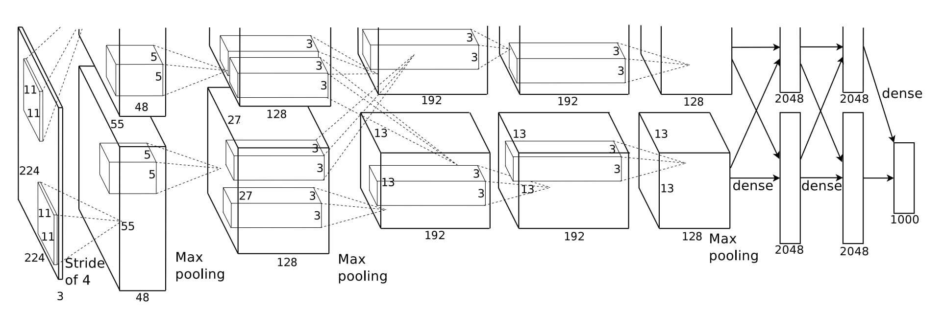Figure 1: AlexNet Architecture

Feature Extraction Layers

The feature extraction part of AlexNet consists of a series of convolutional, normalization, and pooling layers that transform the input image into high-level feature maps.

1. Input Layer

   • Size: 256 × 256 × 3

2. First Convolutional Layer

   • Input filter size: 224 × 224 × 3
   • 96 kernels of size 11 × 11 × 3
   • Stride: 4

3. Second Convolutional Layer

   • Response normalization: k = 2, n = 5, α = 10⁴, β = 0.75
   • Max pooling: kernel size = 3, stride = 2
   • Input size: 11 × 11 × 3
   • 256 kernels of size 5 × 5 × 48
   • Stride: 1

4. Third Convolutional Layer

   • Input size: 5 × 5 × 48
   • 384 kernels of size 3 × 3 × 256
   • Stride: 1

5. Fourth Convolutional Layer

   • Input size: 3 × 3 × 256
   • 384 kernels of size 3 × 3 × 192
   • Stride: 1

6. Fifth Convolutional Layer

   • Input size: 3 × 3 × 192
   • 256 kernels of size 3 × 3 × 192
   • Stride: 1

7. Sixth Layer

   • Max pooling layer: kernel size = 3, stride = 2

Classifier Layers

The classifier layers take the extracted features and produce the final class predictions.

• Dropout: 0.5
• Fully Connected Layer:
  • Input size: 256 × 6 × 6 = 9216
  • Output size: depends on number of classes

Initialization Parameters

Proper initialization is important for stable training:

• Weights for all layers are drawn from a zero-mean Gaussian distribution with standard deviation = 0.01
• Biases:
  • Layers 2, 4, 5 (conv) and fully connected hidden layers: 1
  • Remaining layers: 0

This configuration allows AlexNet to learn hierarchical feature representations effectively, starting from low-level edges and textures to high-level semantic concepts.

Training Details

Optimization

• Optimizer: SGD with momentum (0.9)
• Batch size: 128
• Weight decay: 0.0005
• Learning rate: 0.01, decreased by a factor of 10 when validation error plateaus
• Training time: 5-6 days on two NVIDIA GTX 580 GPUs

Loss Function

Standard cross-entropy loss for multi-class classification:

criterion = nn.CrossEntropyLoss()
optimizer = torch.optim.SGD(model.parameters(), lr=0.01, momentum=0.9, weight_decay=0.0005)

Testing AlexNet Across Training Checkpoints

This test evaluates how an AlexNet model’s predictions evolve over different training epochs. A single test image is loaded and passed through models saved at multiple checkpoints (e.g., after 1, 10, 20, and 30 epochs). For each checkpoint, the model predicts the class of the image, and the results are displayed alongside the original image. This allows visual comparison of how the model’s accuracy and confidence improve as training progresses. 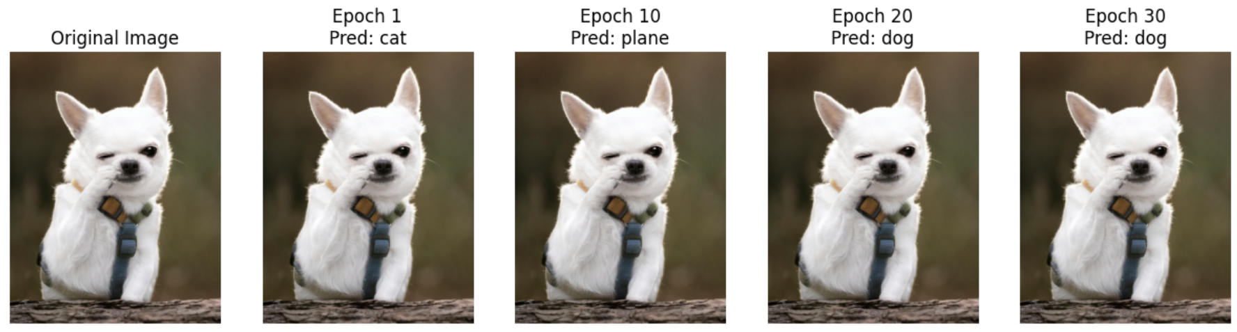Figure 2: Predictions of AlexNet on a test image at different training epochs, showing how model accuracy improves over time.

Feature Map Visualization Across Training Epochs

This visualization shows the intermediate activations (feature maps) from a chosen convolutional layer of AlexNet for a test image. By comparing across different training epochs, you can see how the network gradually learns to extract relevant features, while the probability distribution column shows the model’s confidence in each class prediction.

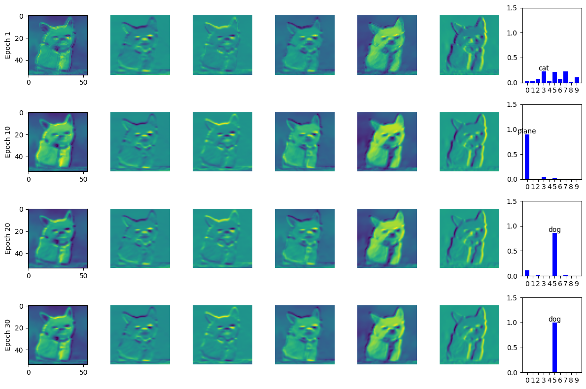Figure 3: Selected convolutional layer feature maps of AlexNet for a test image, showing how learned representations evolve over different epochs alongside the predicted class probabilities.

Conclusion

Building AlexNet from scratch provides valuable insights into the foundations of modern deep learning. Understanding its architecture, training techniques, and innovations helps appreciate how far the field has come while recognizing the enduring principles that continue to guide neural network design today.

The network’s combination of depth, ReLU activations, dropout regularization, and careful initialization created a powerful model that forever changed computer vision and machine learning.