GPT from Scratch - Notes
Learning to build and train transformer-based language models by implementing GPT-2 architecture step by step.
Key Papers:
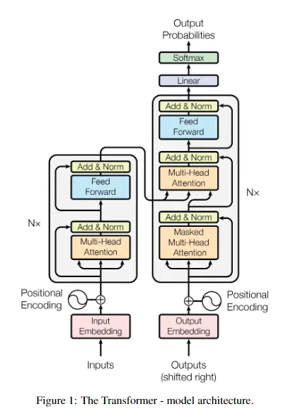
- Attention Is All You Need - Vaswani et al. (2017) - The original Transformer architecture
- Improving Language Understanding by Generative Pre-Training - Radford et al. (2018) - GPT-1
- Language Models are Unsupervised Multitask Learners - Radford et al. (2019) - GPT-2
Tokenization: Why Do We Need It?
Tokenization is the process of converting string data into integers. This allows us to feed text into neural networks.
In this project, we will use character-level encoding and decoding.
# Create a mapping from characters to integers
stoi = {ch:i for i,ch in enumerate(chars)}
itos = {i:ch for i,ch in enumerate(chars)}

encode = lambda s: [stoi[c] for c in s]  # Encoder: string -> list of integers
decode = lambda l: ''.join([itos[i] for i in l])  # Decoder: list of integers -> string

print(encode("hii there"))  # Output: [46, 47, 47, 1, 58, 46, 43, 56, 43]
print(decode(encode("hii there")))  # Output: "hii there"
The above is a simple example. There are more efficient encoding methods, but we will stick to this for the project.
Next, we encode the entire text dataset into a list of integers:
data = torch.tensor(encode(text), dtype=torch.long)
This converts the long text data into a tensor.
Chunks
We never feed the entire text into the model at once (computationally expensive). Instead, we divide the training data into chunks.
block_size = 8
train_data[:block_size+1]  # Output: tensor([18, 47, 56, 57, 58, 1, 15, 47, 58])
block_sizeis the number of tokens considered at a time.- The output
[18, 47, 56, ...]represent a sliding window context for predicting the next character.
Note that the tensor([18, 47, 56, 57, 58, 1, 15, 47, 58]) has multiple examples packed into it and all these characters follow each other. Meaning - if input is [18], the output is likely [47], in the context of [18, 47] the output is [56] and so on all the way up to [18, 47, 56, 57, 58, 1, 15, 47] and the output is likely [58].
So in one pass, we train on all the 8 examples, with content between 1 and block size (here 8), so that the model can understand context everything in between. so the model would predict everything up to block size and then we have to start truncating coz the model would never receiver input size bigger than block size.
Batch dimension: efficiency purpose, parallel processing, multiple chunks at the same time but they are completely independent of each other.
Batch Dimension
We use batching for parallel processing, feeding multiple independent chunks at once.
batch_size = 4
block_size = 8

def get_batch(split):
   # Generate a small batch of input (x) and target (y)
   data = train_data if split == 'train' else val_data
   ix = torch.randint(len(data) - block_size, (batch_size,))
   x = torch.stack([data[i:i+block_size] for i in ix])
   y = torch.stack([data[i+1:i+block_size+1] for i in ix])
   return x, y
The get_batch() function:
ixgenerates random starting positions for our training examples. With a batch size of 4, this creates 4 random offsets, each an integer between0 and len(data) - block_size. These offsets tell us where to start reading from our dataset.xextracts our input sequences. For each offseti, we grabblock_sizeconsecutive characters starting at positioni. The corresponding targetsyare simply the next character after each position inx.torch.stackfunction takes these individual 1-dimensional tensors (one for each offset) and stacks them into a single 2-dimensional tensor with shape(batch_size, block_size). In this case, a 4×8 tensor. Each row represents one independent training sequence.
Bigram Model
BigramLanguageModel() is a custom class that inherits from nn.Module (a PyTorch base class for all neural networks). Note that the super().__init__() calls the constructor of the parent class (nn.Module) to initialize its internals.
class BigramLanguageModel(nn.Module):
   def __init__(self, vocab_size):
       super().__init__()
       # Each token directly predicts the next token from a lookup table
       self.token_embedding_table = nn.Embedding(vocab_size, vocab_size)

   def forward(self, idx, targets=None):
       # idx and targets are (B, T) tensors
       logits = self.token_embedding_table(idx)  # (B, T, C)
       return logits
The Bigram model has the following properties:
nn.Embeddingcreates a lookup table of size(vocab_size, vocab_size).- Input
idxselects rows from the embedding table corresponding to token indices.
So when we pass idx, every single input will refer to the embedding table and is going to select a row of the table corresponding to its index. Example input/output:
print(xb)
# tensor([[24, 43, 58,  5, 57,  1, 46, 43],
#         [44, 53, 56,  1, 58, 46, 39, 58],
#         [52, 58,  1, 58, 46, 39, 58,  1],
#         [25, 17, 27, 10,  0, 21,  1, 54]])
‘24’ will correspond to 24th row in embedding table, similarly ‘5’ will correspond to 5th row. PyTorch then organizes these embeddings into a tensor with shape (batch, time, channel). In our case, that’s (4, 8, 65) — where batch size is 4, time (context length) is 8, and channels equal our vocabulary size of 65.
The line logits = self.token_embedding_table(idx) # (B,T,C) produces logits, which are scores representing the likelihood of each possible next character in the sequence. At this stage, we’re predicting what comes next based solely on the identity of a single token, without considering any surrounding context.
This is why we call it a bigram model. It only looks at pairs of tokens (the current token and the next one). When we initialize and print this model, we see:
m = BigramLanguageModel(vocab_size)
out = m(xb, yb)
print(out.shape)
# torch.Size([4, 8, 65])
That is, out contains the logits for each token in the sequence for each item in the batch.
for example, out[0][0] would give the logits for the next token prediction for the first token in the first sequence, and out[1][2] would give the logits for the third token in the second sequence.
B, T, C = logits.shape
            logits = logits.view(B*T, C)
            targets = targets.view(B*T)
            loss = F.cross_entropy(logits, targets)
Reshaping for the Loss Function
PyTorch’s cross-entropy loss expects the channel dimension (C) as the second argument, with the format (N, C) where N is the number of predictions. However, our logits currently have shape (B, T, C)—batch, time, and channel.
To conform to PyTorch’s requirements, we need to reshape our tensors. We unpack the batch and time dimensions by flattening them into a single dimension, transforming our (B, T, C) tensor into (B*T, C). This way, the channel dimension C becomes the second argument as expected.
For the targets, we apply a similar transformation—converting our (B, T) tensor into a 1-dimensional tensor of length B*T. We can accomplish this efficiently using targets.view(-1), which flattens the tensor while letting PyTorch infer the correct size automatically.
m = BigramLanguageModel(vocab_size)
logits, loss = m(xb, yb)
print(logits.shape)
print(loss)

'''
output:
torch.Size([32, 65])
tensor(4.8786, grad_fn=<NllLossBackward0>)
'''
Since our vocabulary size is 65, we’d expect the initial loss from a completely untrained model to be around -ln(1/65) ≈ 4.17. This represents maximum entropy—the model guessing uniformly at random across all possible tokens.
Our actual loss of 4.88 is slightly higher than this theoretical baseline, which is normal for randomly initialized weights. The model’s initial predictions are essentially random, containing high entropy. As training progresses, we expect this loss to decrease as the model learns meaningful patterns in the data.
How text generation works
The generate() function takes idx, a tensor of shape (B, T) representing the current context—B sequences of T tokens each—and extends each sequence by max_new_tokens new characters.
def generate(self, idx, max_new_tokens):
    # idx is (B, T) array of token indices
    for _ in range(max_new_tokens):
        logits, loss = self(idx)
        logits = logits[:, -1, :]  # Focus on last time step (B, C)
        probs = F.softmax(logits, dim=-1)  # Convert logits to probabilities
        idx_next = torch.multinomial(probs, num_samples=1)  # Sample next token
        idx = torch.cat((idx, idx_next), dim=1)  # Append to running sequence
    return idx
Here’s the step-by-step process:
- Get predictions: We pass the current context through the model to get logits for all time steps
- Focus on the last position: We extract only the logits at the final time step using
logits[:, -1, :], giving us shape(B, C)—predictions for what should come next - Convert to probabilities: We apply softmax to transform raw logits into a probability distribution over the vocabulary
- Sample the next token: Using
torch.multinomial(), we randomly sample one token from this distribution for each batch element, producing a tensor of shape(B, 1) - Extend the context: We concatenate the newly sampled token to our running sequence, expanding it from
(B, T)to(B, T+1)
This process repeats for max_new_tokens iterations, with each new token becoming part of the context for predicting the next one.
GPT-2 Skeleton
This structure mirrors the GPT-2 paper’s architecture diagram:
wte(token embeddings): Maps each token in the vocabulary to a learned embedding vector of dimensionn_embd(768 in GPT-2 124M)wpe(positional embeddings): Encodes the position of each token in the sequence, up toblock_sizepositionsh(transformer blocks): A stack ofn_layeridentical transformer blocks (12 layers in GPT-2 124M), shown as the gray blocks in the architecture diagramln_f(final layer norm): A layer normalization applied after all transformer blocks—this is a GPT-2 specific addition not present in the original GPTlm_head(language modeling head): The final linear layer that projects from the embedding dimension (768) back to vocabulary size (50,257 for GPT-2), producing logits for next-token prediction
The architecture is shown below: